If you did not find the geospatial data you need in existing R packages (see the map section), you need to find this information elsewhere on the web.

It will often be stored as a .geomJSON format. This post explains how to read it.

Note: if you found a shapefile, read this post instead.

Find and download a .geoJSON file

You need to dig the internet to find the geoJSON file you are interested in. For instance, this URL provides a file containing french region boundaries.

You can load it in R with:

# Let's read the jeoJson file that is stored on the web with the geojsonio library:
library(geojsonio)
spdf <- geojson_read("https://raw.githubusercontent.com/gregoiredavid/france-geojson/master/communes.geojson",  what = "sp")

That’s it! You now have a geospatial object called spdf. I strongly advise to read this post to learn how to manipulate it.

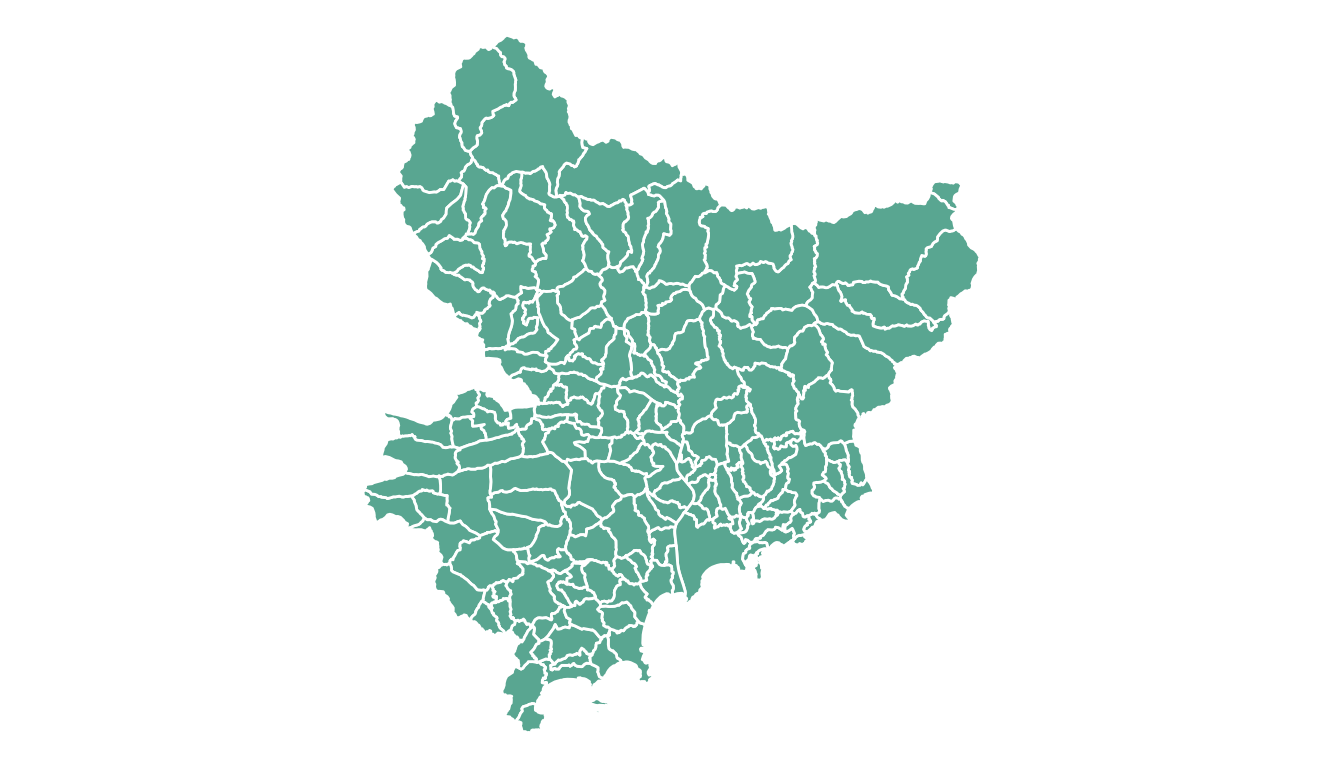
Just in case, here is how to plot it in base R and with ggplot2.

Plot it with base R

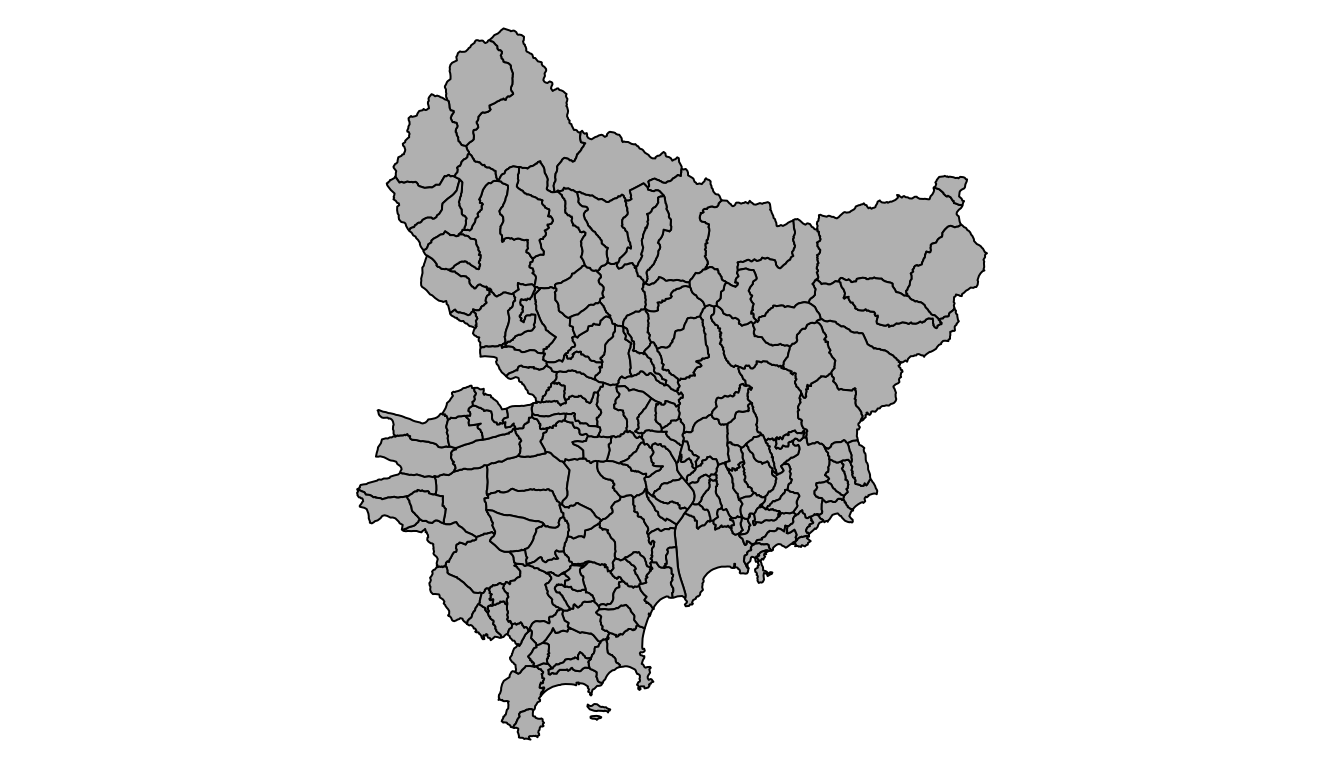
# Select only the region #6
spdf@data$mystate = substr( spdf@data$code, 1, 2)
spdf_region_6 = spdf[ spdf@data$mystate == "06" , ]

# plot the selected are with sp
library(sp)
par(mar=c(0,0,0,0))
plot(spdf_region_6, col="grey")

Plot it with ggplot2

# 'fortify' the data to get a dataframe format required by ggplot2
library(broom)
spdf_fortified <- tidy(spdf_region_6)

# Plot it
library(ggplot2)
ggplot() +
  geom_polygon(data = spdf_fortified, aes( x = long, y = lat, group = group), fill="#69b3a2", color="white") +
  theme_void() +
  coord_map()